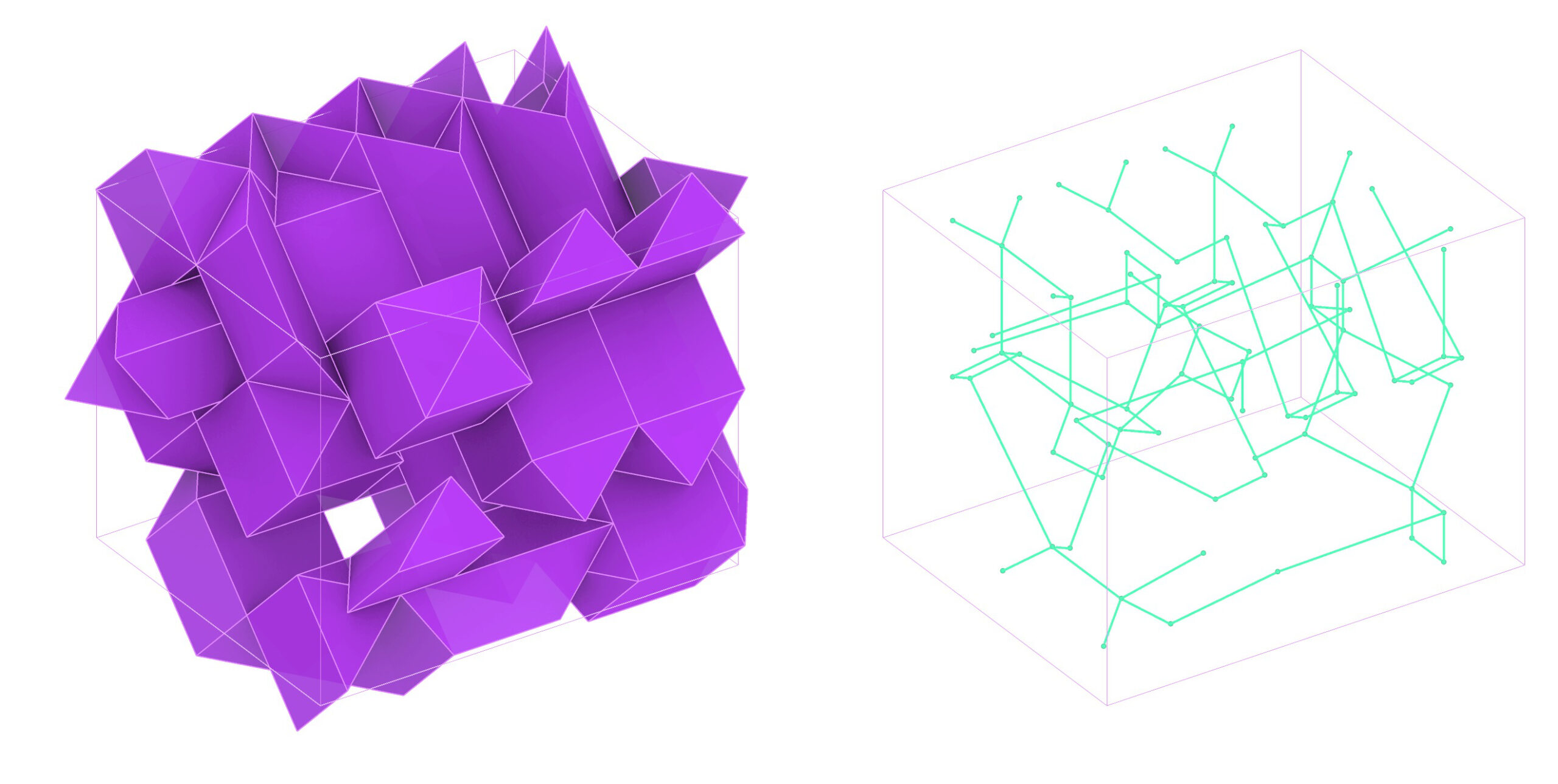
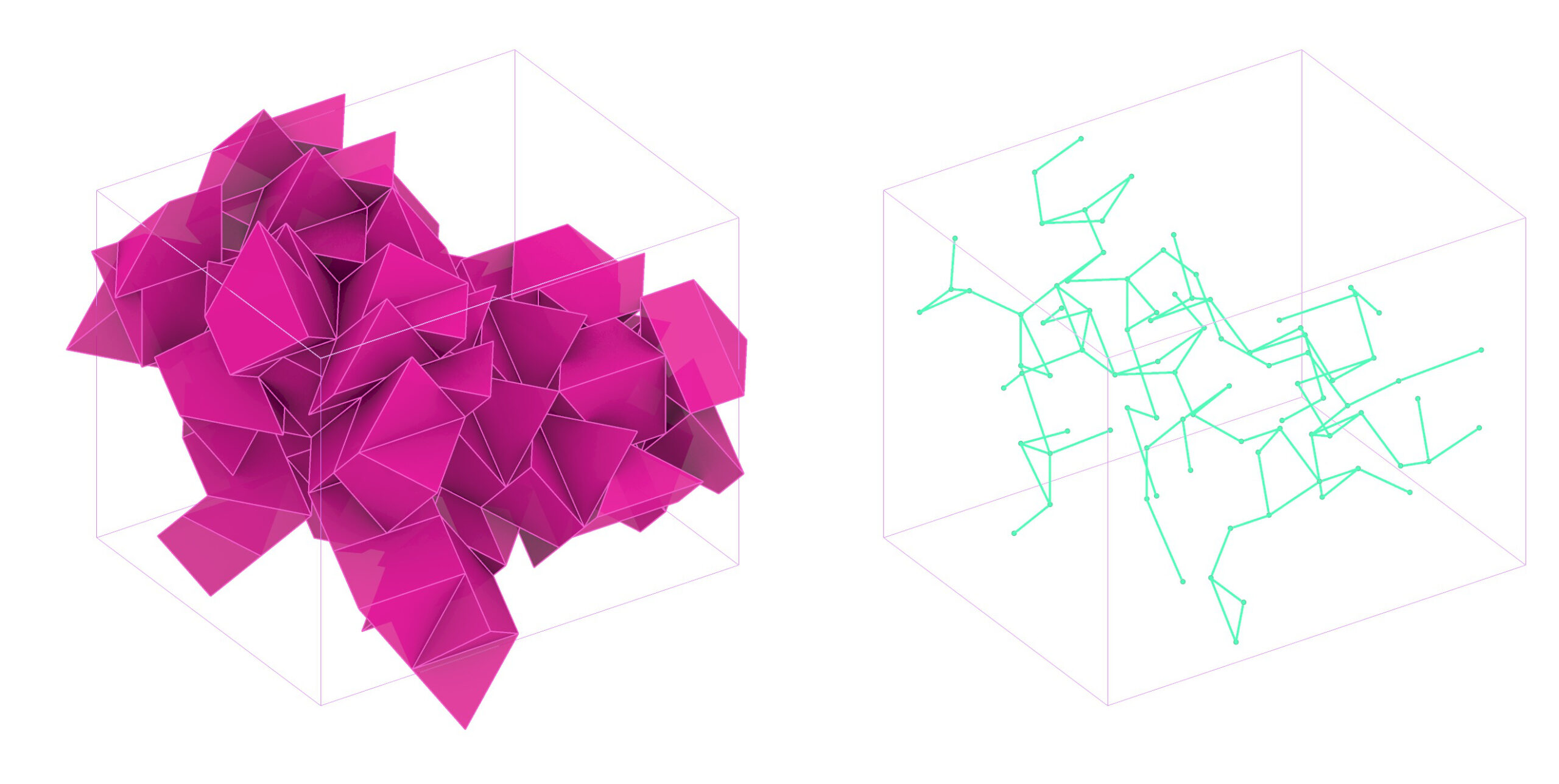
Manual for a discrete element aggregation of volumetric parts based on tetrahedral geometry using the Wasp plugin for Grasshopper in Rhinoceros.
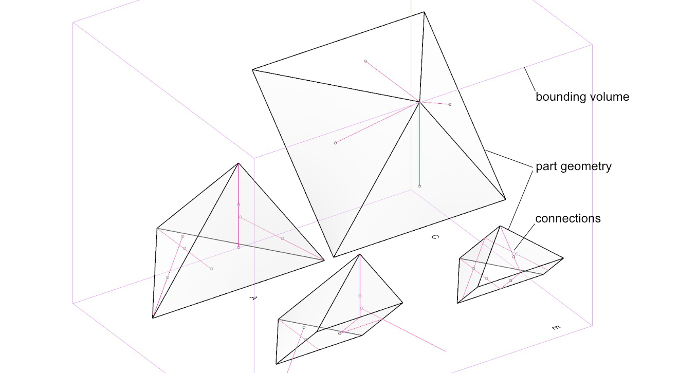
This definition uses a collection of geometries that are derived from a space-filling tetrahedron called Sommerville no.1, for more details have a look at this previous post.
In the study Sommerville – Multiple Part Types, we experimented with variations of the original tetrahedral geometry as parts for discrete aggregation. We found that specific subdivisions and combinations of fragments of a Sommerville tetrahedron produce different compatible forms that can be aggregated to interconnected structures.
This file set provides a template for testing aggregations of up to 4 volumetric part types (without the inscribed bicycle frame geometry we used in the previous study)
The definition is structured in 3 sections:
- module parts
- aggregation
- output
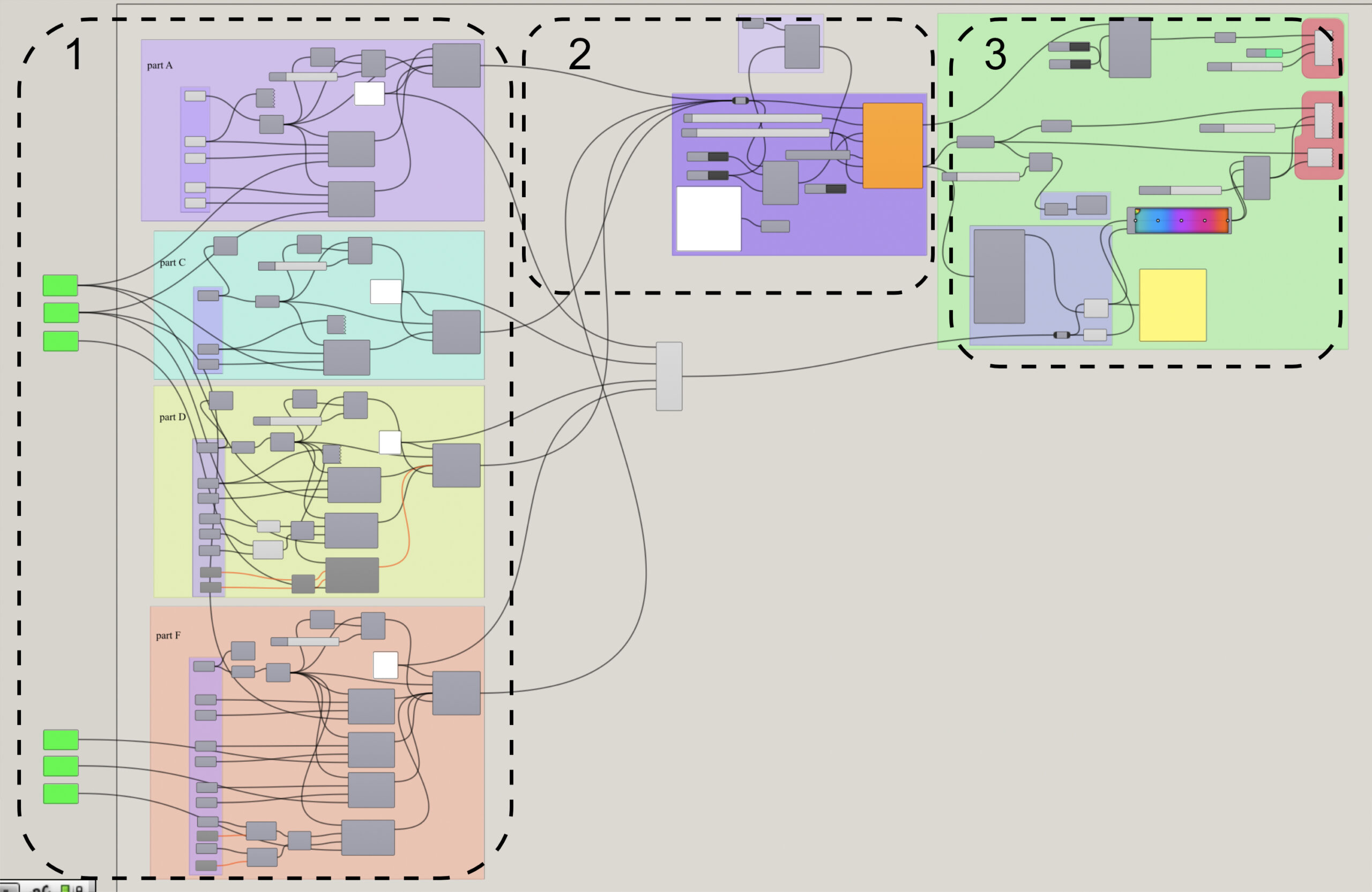
In section 1, the four solid types (each in a box with a different color) are compiled as Wasp parts based on geometry referenced from the Rhino workspace. Connections are set at the faces of the volumes.
Different numbers are assigned to the part connections as “connection type” to differentiate the compatibility between parts (green boxes at the far left), only connections of the same type are used for aggregation.
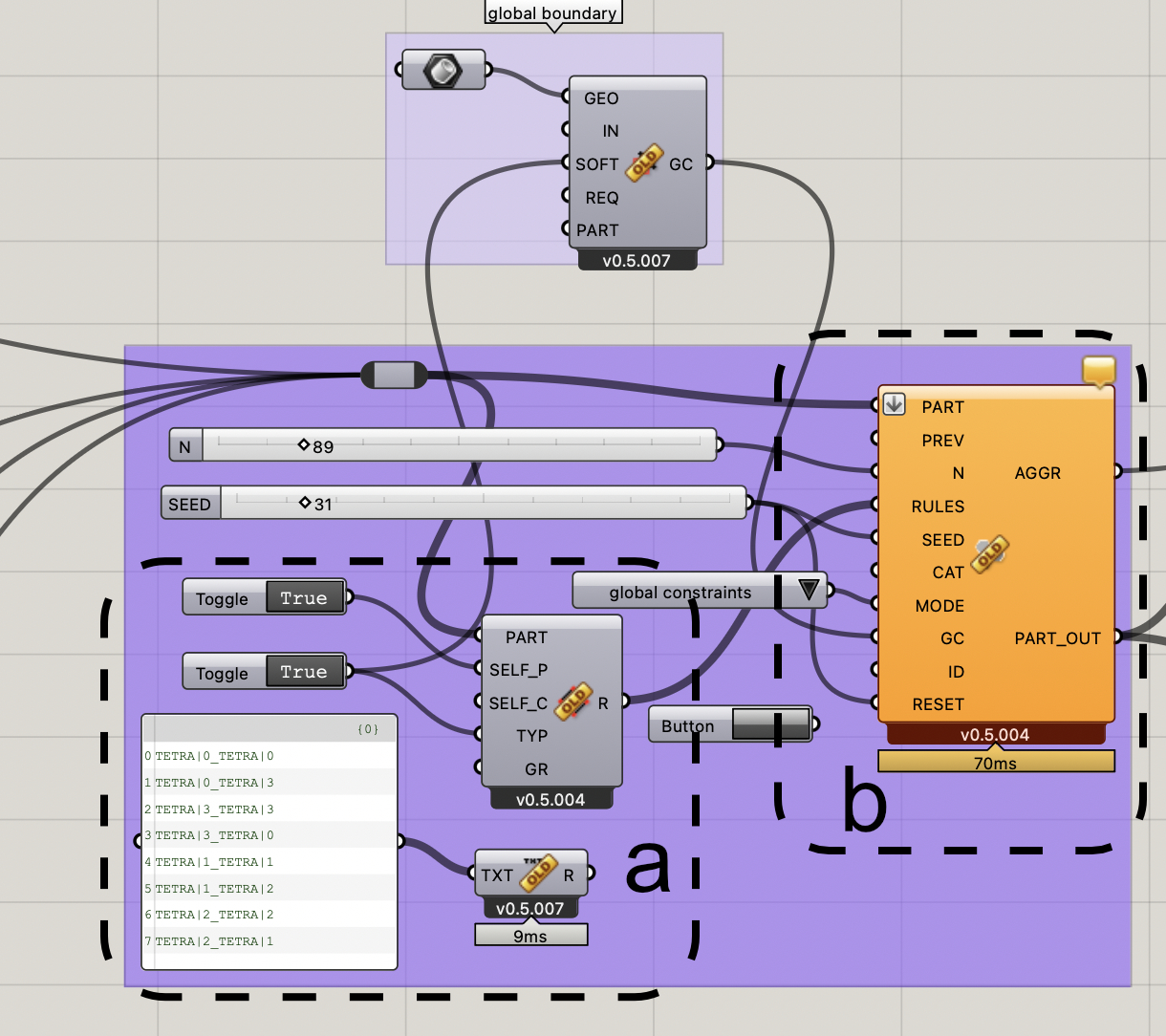
In section 2, aggregation rules are automatically generated from the set of parts including connections (a). With the input at “TYP” set to “true”, only rules for connections of the same type are allowed.
In section 2b, an aggregation is compiled. The input “MODE” allows to constrain the aggregation within a bounding volume, setting it to “no constraints” removes this restriction. With “N” you can set the amount of parts and “SEED” controls the versions of random constellations.
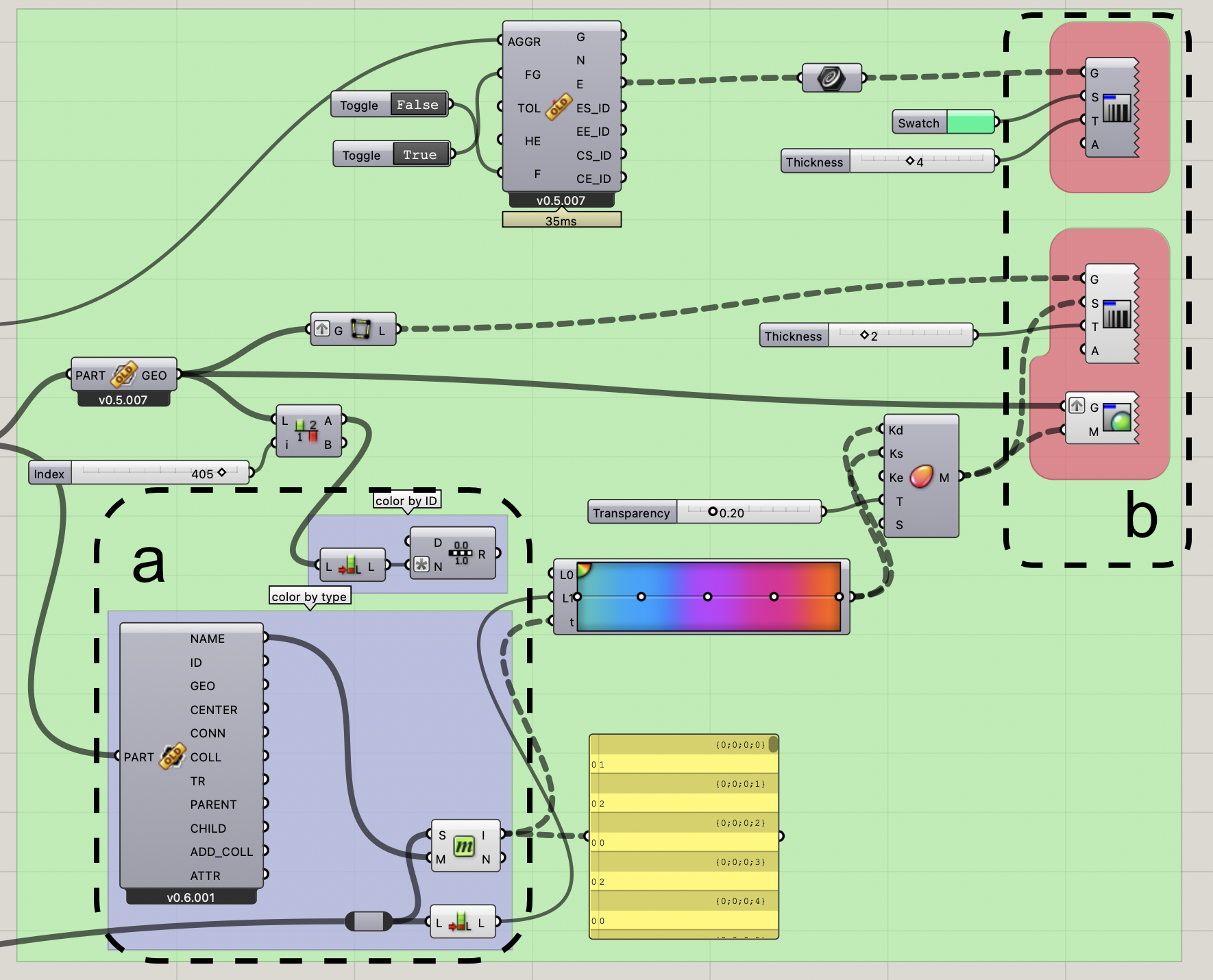
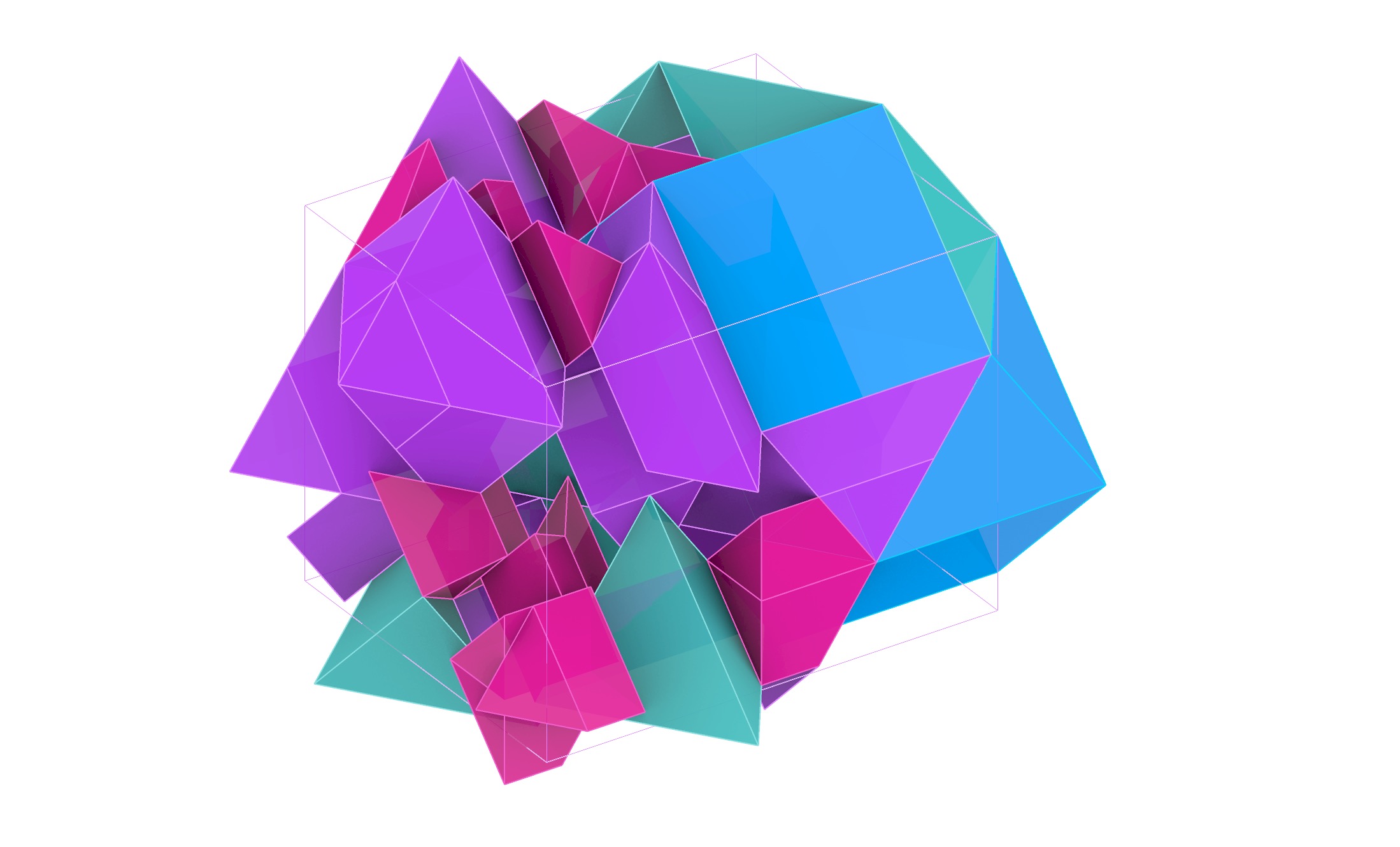
In section 3, output geometry can be displayed. Colors can be set by part instance or by part type (a). At the far right, in the red boxes, part geometries and the aggregation graph can be displayed (b).
The component at the right top inside the red box (b) displays the connection graph. Besides aligning connections parts do also meet at co-planar faces where no connections are defined, but in the graph only those aligning connections are visible. Therefore, in this case, the graph is not a comprehensive representation of all possible connections in the structure if aligning faces were considered connected.

Since all parts are based on logical subdivisions or multiplications of the basic Sommerville Tetrahedron unit, the resulting aggregations behave like a strange fractal structure able to shift in between scales of parts. Unlike in a truly fractal system, the part geometry varies from one scale to another, but the different forms relate to one another which makes them compatible – stochastic aggregation sequences can form spontaneous interconnections, close open ends and (locally) produce cellular structures.
To increase the likeliness of interconnections you could play with additional connections that would further increase part connectivity.
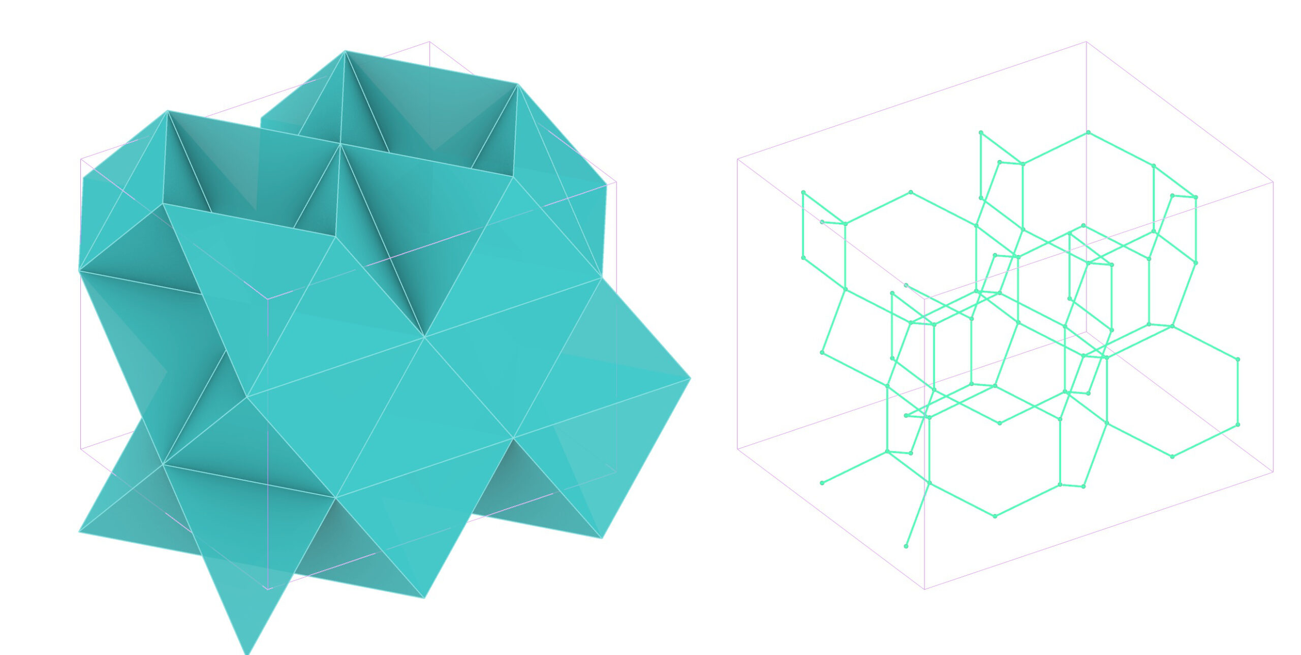
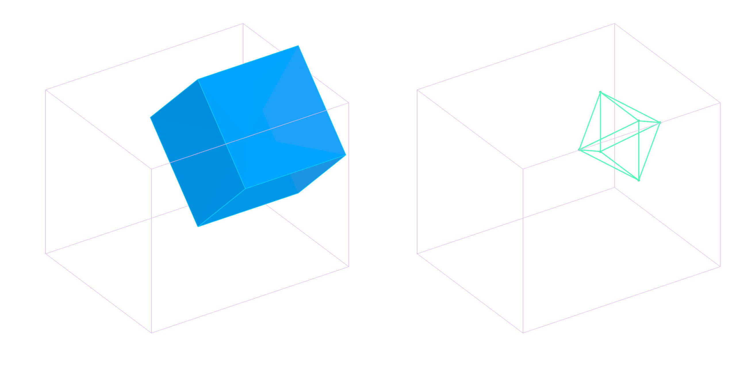
Because for part C, no connections are defined at the square face at the base of the geometry, an aggregation only with this type is limited to 6 parts, resulting in a cube.